SE-PINN
Solving the Schrödinger Equation via Physics-Informed Machine Learning
Introduction
SE-PINN is a physics-informed neural network in PyTorch that solves the Schrödinger equation of quantum mechanics.
Here, I first explain how SE-PINN is designed and then demonstrate how SE-PINN is applied to the quantum harmonic oscillator, which is a model that is used for the interatomic bonding of molecules such as hydrogen iodide and hydrogen fluoride.
How SE-PINN is Designed
As a physics-informed neural network (PINN), SE-PINN uses principles from physics to reduce the space of solutions in which it searches.
In particular, four physical constraints are used: normality, orthogonality, symmetry, and consistency, all of which are explained in the subsequent sections.
Each physical constraint is integrated into SE-PINN through one of two methods: (1) inclusion in the objective function of the model (which is used for normality, orthogonality, and consistency) or (2) exact conservation via the architecture of the model (which is used for symmetry).
An outstanding feature of SE-PINN is that it is not trained on a set of labeled examples — in other words via supervised learning. In contrast, it learns via reinforcement learning (RL) through direct feedback from the SE, which enables it to adapt to any quantum-mechanical system.
In fact, it is a minimal example of RL, defined by the Markov Decision Process (MDP) in which the state is the parameters of the model, the action is to compute its predictions based on the parameters, the instantaneous total reward is the negation of the loss, and the policy is to update the parameters to minimize the loss.
In addition, SE-PINN is trained with the L-BFGS algorithm, which is a second-order optimizer that approximates the Hessian matrix.
Last, SE-PINN is organized into two classes: BasePINN, which implements the architecture of the model, and PINN, which is a wrapper of BasePINN that includes infrastructure for training and visualization.
The decoupling of the design enables users to define custom classes that change or extend SE-PINN.
Background
(1) Physics
Quantum mechanics is a theory of physics at the atomic scale.
The central equation of quantum mechanics is the Schrödinger equation, whose time-independent form is as follows.
\[ - \frac{\hbar^{2}}{2m} \frac{d^2\psi}{dx^2} + V \psi = E \psi \]
- \(\hbar\) is the reduced Planck constant.
- \(m\) is the mass of the system.
- \(\psi\) is the wavefunction of the system.
- \(x\) is the spatial coordinate (position).
- \(V\) is the potential-energy field of the system.
- \(E\) is the energy of the system.
\(\psi\), the wavefunction of the system, is the representation of its state.
In classical mechanics, physical quantities such as position and momentum can be measured with infinite precision (in theory). In quantum mechanics, however, the wavefunction is an intermediary between physical quantities and measurements of them.
Heisenberg’s uncertainty principle, for example, indicates that simultaneous measurements of position and momentum are limited in precision.
(2) Mathematics
Matrices of complex numbers are central in quantum mechanics.
The complex conjugate, \(z^{*}\), of a complex number, \(z\), is the complex number whose real part is identical and whose imaginary part is equal in magnitude and opposite in sign. In other words, the complex conjugate of \(a + bi\) is \(a - bi\), and vice versa.
The modulus, \(|z|\), of a complex number, \(z = a + bi\), is equal to \(\sqrt{a^2 + b^2}\). Moreover, the square of the modulus is equal to the product of \(z\) and its complex conjugate: \(|z|^2 = z^{*}z\).
The conjugate transpose, \(A^{*}\), of a complex matrix, \(A\), is its transpose where each element is instead its complex conjugate.
A Hermitian matrix is a matrix that is equal to its conjugate transpose. In other words, \(A = A^{*}\).
Extension of modulus to complex vectors / matrices.
Property 1: Normality
Physics: In the Copenhagen interpretation of quantum mechanics, the wavefunction of a physical system determines the probability that the system is observed to be in a particular state. In particular, the squared modulus of the wavefunction, \(|\psi(x)|^{2}\), is a probability density function.
\[\int_{a}^{b} |\psi(x)|^{2} \,dx = \Pr[a \leq X \leq b]\]
Mathematics: The integral of such a quantity over all states must be equal to 1 due to the law of total probability. Furthermore, for systems that are bound to a potential and therefore localized in space, the limit of the wavefunction at infinity must be equal to 0.
\[\int_{-\infty}^{+\infty} |\psi(x)|^{2} \,dx = 1\]
\[ \lim_{x\to\pm\infty} \psi(x) = 0 \]
SE-PINN: The objective function of the model includes both a normality-based component that is adjusted for discretization (dx) and a boundary-based component.
normality_loss = (torch.sum(wf ** 2) - 1 / self.dx) ** 2Derivation
\[\begin{equation} \begin{split} \int_{-\infty}^{+\infty} |\psi(x)|^{2} \,dx & = 1 \\[1em] \sum_{i} |\psi(x_{i})|^{2} \,\Delta x & = 1 \\[1em] \sum_{i} |\psi(x_{i})|^{2} & = \frac{1}{\Delta x} \\[1em] \sum_{i} |\psi(x_{i})|^{2} - \frac{1}{\Delta x} & = 0 \\[1em] \left( \sum_{i} |\psi(x_{i})|^{2} - \frac{1}{\Delta x} \right)^{2} & = 0 \end{split} \end{equation}\]
Explanation
The final squaring is used so that positive values and negative values are additive rather than subtractive and so that high values are penalized more. But another function such as the absolute value can be used as well.
Moreover, such a loss discourages trivial solutions (wavefunctions of 0) since they result in non-zero loss, \(\left(\frac{1}{\Delta x}\right)^{2}\), while non-trivial solutions result in zero loss.
boundary_loss = wf[0] ** 2 + wf[-1] ** 2Explanation
wf[0] is the value at the left end of the wavefunction, and wf[-1] is the value at the right end of the wavefunction.
The squaring of each end is used so that (1) positive values and negative values are additive rather than subtractive and (2) high values are penalized more.
Property 2: Orthogonality
Physics: Measurements of a physical quantity, such as energy, are real numbers rather than complex numbers.
\[E \in \mathbb{R}\]
Mathematics: Measurements of a physical quantity are eigenvalues of a complex matrix that represents the physical quantity. Since these eigenvalues are real, the matrix must be Hermitian. Thus, as a property of Hermitian matrices, the set of all eigenvectors of such a matrix must be an orthogonal set; in other words, every eigenvector must be orthogonal to every other eigenvector.
\[ \psi_{i}(x)^{*} \psi_{j}(x) = 0, \ i \neq j\]
Proof
The proof follows from the fact that the Hamiltonian matrix, \(H\), is Hermitian (\(H = H^{*}\)), that the indices of the eigenvectors are distinct (\(i \neq j\)), and that the eigenvalues of such eigenvectors are non-degenerate (\(E_{i} \neq E_{j}\)).
\[\begin{equation} \begin{split} \psi_{i}(x)^{*} \hat{H}^{*} \psi_{j}(x) & = \psi_{i}(x)^{*} \hat{H}^{*} \psi_{j}(x) \\[1em] \left(\hat{H} \psi_{i}(x)\right)^{*} \psi_{j}(x) & = \psi_{i}(x)^{*} \left(\hat{H} \psi_{j}(x)\right) \\[1em] E_{i} \left(\psi_{i}(x)^{*} \psi_{j}(x)\right) & = E_{j} \left(\psi_{i}(x)^{*} \psi_{j}(x)\right) \\[1em] E_{i} \left(\psi_{i}(x)^{*} \psi_{j}(x)\right) - E_{j} \left(\psi_{i}(x)^{*} \psi_{j}(x)\right) & = 0 \\[1em] (E_{i} - E_{j}) \left(\psi_{i}(x)^{*} \psi_{j}(x)\right) & = 0 \\[1em] \psi_{i}(x)^{*} \psi_{j}(x) & = 0 \end{split} \end{equation}\]
SE-PINN: The objective function of the model includes an orthogonality-based component.
orthogonality_loss = torch.dot(wf, self.basis_sum) ** 2Explanation
self.basis_sum is the sum of all other eigenvectors so far learned by SE-PINN, and it is therefore a linear combination of these eigenvectors. As a result, any vector that is orthogonal to self.basis_sum is orthogonal to each of the other eigenvectors. The great advantage is that computing the inner product of the current wavefunction and self.basis_sum is much more efficient than computing it for each pair.
The final squaring is used so that positive values and negative values are additive rather than subtractive and so that high values are penalized more. But another function such as the absolute value can be used as well.
Property 3: Symmetry
Physics: If the quantum-mechanical potential of a system is even, in other words symmetric about the y-axis such that \(V(x) = V(-x)\), then the eigenvectors of energy that are bound to the potential are also symmetric, either even or odd.
Proof
The proof follows from the Schrödinger equation.
\[\begin{equation} \begin{split} - \frac{\hbar^{2}}{2m} \frac{d^2\psi(x)}{dx^2} + V(x) \psi(x) & = E \psi(x) \\[1em] - \frac{\hbar^{2}}{2m} \frac{d^2\psi(-x)}{d(-x)^2} + V(-x) \psi(-x) & = E \psi(-x) \\[1em] - \frac{\hbar^{2}}{2m} \frac{d^2\psi(-x)}{dx^2} + V(x) \psi(-x) & = E \psi(-x) \end{split} \end{equation}\]
Thus, both \(\psi(x)\) and \(\psi(-x)\) are solutions of the same energy, \(E\).
However, since eigenvectors that are bound to the potential are non-degenerate, \(\psi(x)\) and \(\psi(-x)\) correspond to the same solution.
Moreover, since the Schrödinger equation is a linear equation, \(\psi(x) = a \psi(-x)\), and both \(a = 1\) and \(a = -1\) are valid.
As a result, \(\psi(x) = \psi(-x)\) is an even solution, \(\psi(x) = -\psi(-x)\) is an odd solution, and every solution is either even or odd.
Mathematics: Any function whose domain is symmetric about the origin can be expressed as the sum of an even function and an odd function, and therefore these components can be separated.
\[ \psi_{\text{E}}(x) = \frac{1}{2} (\psi(x) + \psi(-x)) \]
\[ \psi_{\text{O}}(x) = \frac{1}{2} (\psi(x) - \psi(-x)) \]
\[ \psi(x) = \psi_{\text{E}}(x) + \psi_{\text{O}}(x) \]
Proof
As indicated above, the domain of \(\psi(x)\) must be symmetric about the origin for such a decomposition to exist. Otherwise \(\psi(-x)\) is not defined for all values of \(x\) in the domain!
- \(\psi_{\text{E}}(x) + \psi_{\text{O}}(x)\) is a decomposition of \(\psi(x)\).
\[\begin{equation} \begin{split} \psi_{\text{E}}(x) + \psi_{\text{O}}(x) & = \frac{1}{2} (\psi(x) + \psi(-x)) + \frac{1}{2} (\psi(x) - \psi(-x)) \\[1em] & = \frac{1}{2} \psi(x) + \frac{1}{2} \psi(-x) + \frac{1}{2} \psi(x) - \frac{1}{2} \psi(-x) \\[1em] & = \psi(x) \end{split} \end{equation}\]
- \(\psi_{\text{E}}(x)\) is even.
\[\begin{equation} \begin{split} \psi_{\text{E}}(x) & = \frac{1}{2} (\psi(x) + \psi(-x)) \\[1em] & = \frac{1}{2} (\psi(-x) + \psi(x)) \\[1em] & = \psi_{\text{E}}(-x) \end{split} \end{equation}\]
- \(\psi_{\text{O}}(x)\) is odd.
\[\begin{equation} \begin{split} \psi_{\text{O}}(x) & = \frac{1}{2} (\psi(x) - \psi(-x)) \\[1em] & = -\frac{1}{2} (\psi(-x) - \psi(x)) \\[1em] & = -\psi_{\text{O}}(-x) \end{split} \end{equation}\]
SE-PINN: A custom architectural layer that can enforce such a separation — a hub layer — is used as the final layer of the model.
predicted_wf = self.even * 0.5 * (torch.mm(self.weights, H_plus) + 2 * self.bias)
             + self.odd * 0.5 * torch.mm(self.weights, H_minus)
Derivation
\[\psi(x) = \sum_{i = 1}^{N} w_{i} h_{i}(x) + b\]
\[\begin{equation} \begin{split} \psi_{\text{E}}(x) & = \frac{1}{2} (\psi(x) + \psi(-x)) \\[1em] & = \frac{1}{2} \left(\sum_{i = 1}^{N} w_{i} h_{i}(x) + b + \sum_{i = 1}^{N} w_{i} h_{i}(-x) + b\right) \\[1em] & = \frac{1}{2} \left(\sum_{i = 1}^{N} (w_{i} h_{i}(x) + w_{i} h_{i}(-x)) + 2 b\right) \\[1em] & = \frac{1}{2} \left(\sum_{i = 1}^{N} w_{i} (h_{i}(x) + h_{i}(-x)) + 2 b\right) \\[1em] & = \frac{1}{2} \left(\sum_{i = 1}^{N} w_{i} H_{i}^{+}(x) + 2 b\right) \end{split} \end{equation}\]
\[\begin{equation} \begin{split} \psi_{\text{O}}(x) & = \frac{1}{2} (\psi(x) - \psi(-x)) \\[1em] & = \frac{1}{2} \left(\sum_{i = 1}^{N} w_{i} h_{i}(x) + b - \left(\sum_{i = 1}^{N} w_{i} h_{i}(-x) + b\right)\right) \\[1em] & = \frac{1}{2} \left(\sum_{i = 1}^{N} (w_{i} h_{i}(x) - w_{i} h_{i}(-x))\right) \\[1em] & = \frac{1}{2} \left(\sum_{i = 1}^{N} w_{i} (h_{i}(x) - h_{i}(-x))\right) \\[1em] & = \frac{1}{2} \left(\sum_{i = 1}^{N} w_{i} H_{i}^{-}(x)\right) \end{split} \end{equation}\]
\[\begin{equation} \begin{split} \psi(x) & = \psi_{\text{E}}(x) + \psi_{\text{O}}(x) \\[1em] & = \frac{1}{2} \left(\sum_{i = 1}^{N} w_{i} H_{i}^{+}(x) + 2 b\right) + \frac{1}{2} \left(\sum_{i = 1}^{N} w_{i} H_{i}^{-}(x)\right) \end{split} \end{equation}\]
Explanation
self.even and self.odd can be configured as 0 or 1 to enforce a particular symmetry.
Since SE-PINN is a neural network, \(\psi(x) = \sum_{i = 1}^{N} w_{i} h_{i}(x) + b\), where \(w_{i}\) is a weight of the final hidden layer, \(h_{i}(x)\) is an input from the previous layer, and \(b\) is the bias of the output layer (a single node).
H_plus and H_minus are used to abbreviate the notation.
H_plus is equal to \(h(x) + h(-x)\), and H_minus is equal to \(h(x) - h(-x)\).
Property 4: Consistency
Physics: Any state of a quantum-mechanical system must satisfy the Schrödinger equation.
Mathematics: The time-independent Schrödinger equation is a differential equation, whose solutions, \(\psi\), are eigenvectors of the Hamiltonian matrix, \(\hat{H} = - \frac{\hbar^{2}}{2m} \frac{d^2}{dx^2} + V\).
\[\begin{equation} \begin{split} \hat{H} \psi & = E \psi \\[1em] - \frac{\hbar^{2}}{2m} \frac{d^2\psi}{dx^2} + V \psi & = E \psi \end{split} \end{equation}\]
SE-PINN: The objective function of the model includes a component that quantifies how well it satisfies the Schrödinger equation via the mean squared error (MSE).
SE_loss = torch.mean((-hbar / (2 * self.m) * dd + self.V * wf - energy * wf) ** 2)Derivation
\(\hbar^{2}\) and \(m\) can be omitted for simplicity and absorbed by \(E\).
\[\begin{equation} \begin{split} - \frac{1}{2} \frac{d^2\psi}{dx^2} + V \psi & = E \psi \\[1em] - \frac{1}{2} \frac{d^2\psi}{dx^2} + V \psi - E \psi & = 0 \\[1em] \end{split} \end{equation}\]
Explanation
dd is the second derivative of the wavefunction with respect to position and is of the same shape as the wavefunction. The potential, self.V, is a scalar-valued function, and energy is a scalar, so self.V * wf and energy * wf are element-wise products.
How SE-PINN is Applied
Step 1: Initialize the Environment
%config InlineBackend.print_figure_kwargs = {'bbox_inches': None}

import os
import random
import sys

import IPython
from matplotlib.animation import FuncAnimation, PillowWriter
import matplotlib_inline
import matplotlib.pyplot as plt
import numpy as np
from rich.progress import (
    BarColumn,
    Progress,
    TaskProgressColumn,
    TextColumn,
    TimeRemainingColumn,
    track
)
from scipy.linalg import eigh_tridiagonal
import torch
import torch.nn as nn

matplotlib_inline.backend_inline.set_matplotlib_formats('retina')
plt.rcParams['figure.figsize'] = (6.4, 4.8)

# Environment Variables
if 'google.colab' not in sys.modules:
    !export LC_ALL='en_US.UTF-8'
    !export LD_LIBRARY_PATH='/usr/lib64-nvidia'
    !export LIBRARY_PATH='/usr/local/cuda/lib64/stubs'

# Optional Hardware Acceleration
# Use Runtime > Change runtime type > T4 GPU on Google Colab.
if torch.cuda.is_available():
    torch.cuda.init()
    torch.cuda.is_initialized()
    torch.set_default_tensor_type('torch.cuda.FloatTensor')
    device = 'cuda'
else:
    device = 'cpu'
device = torch.device(device)
print(f'Using {device}.')

# Settings for Reproducibility
torch.manual_seed(0)
torch.backends.cudnn.benchmark = False
torch.use_deterministic_algorithms(True)
torch.utils.deterministic.fill_uninitialized_memory = True
os.environ['CUBLAS_WORKSPACE_CONFIG']=':4096:2' # cuBLAS
np.random.seed(0)
random.seed(0)

# Convenience Function for Plotting with PyTorch Tensors
def to_plot(x): return x.detach().cpu().numpy()
Step 2: Define the BasePINN Class
class BasePINN(nn.Module):
    """
    A base class for a physics-informed neural network (PINN) for
    solving the Schrodinger equation.

    Attributes
    ----------
    x0 : float
        The spatial position of the leftmost point of the
        quantum-mechanical potential.
    xN : float
        The spatial position of the rightmost point of the
        quantum-mechanical potential.
    dx : float
        The uniform spatial Euclidean distance between adjacent points.
    N : int
        The count of points of the quantum-mechanical potential.
    activation : builtin_function_or_method
        The activation function.
    sym : int
        Whether to enforce even symmetry (1) or odd symmetry (-1) or not
        to enforce symmetry (0).

    Methods
    -------
    swap_symmetry
        Swap the symmetry of the prediction of the model between even
        symmetry and odd symmetry.

    forward(x)
        Forward pass.
    """

    def __init__(self, grid_params, activation, sym=0):
        super(BasePINN, self).__init__()

        self.x0, self.xN, self.dx, self.N = grid_params
        self.activation = activation
        self.sym = sym

        # Architecture of the Model

        self.energy_node = nn.Linear(1, 1)

        self.fc1_bypass = nn.Linear(1, 50)
        self.fc1 = nn.Linear(2, 50)
        self.fc2 = nn.Linear(50, 50)

        # Selection of the Output Layer
        if sym == 1:
            # Enforcement of Even Symmetry
            self.output_layer = HubLayer(50, 1, 1, 0)
        elif sym == -1:
            # Enforcement of Odd Symmetry
            self.output_layer = HubLayer(50, 1, 0, 1)
        else:
            # No Enforcement of Symmetry
            self.output_layer = nn.Linear(50, 1)

    def swap_symmetry(self):
        if self.sym == 0:
            print('Symmetry cannot be swapped because it is not enforced.')
            return
        self.output_layer.flip_sym()

    def forward(self, x):
        # Lambda Layer for Energy
        energy = self.energy_node(torch.ones_like(x))

        N = torch.cat((x, energy), dim=1)
        N = self.activation(self.fc1(N))
        N = self.activation(self.fc2(N))
        wf = self.output_layer(N) # Possible enforcement of symmetry.

        return wf, energy

class HubLayer(nn.Module):
    """
    A hub layer, which is used to constrain the prediction of the model
    to respect even symmetry (symmetry about f(x) = 0) or odd symmetry
    (symmetry about f(x) = x). The mathematical basis is presented at
    https://arxiv.org/pdf/1904.08991.pdf. The constructor is adapted
    from https://auro-227.medium.com/writing-a-custom-layer-in-pytorch-14ab6ac94b77.

    Attributes
    ----------
    size_in : int
        The length of the input of the layer.
    size_out : int
        The length of the output of the layer.
    weights : torch.nn.parameter.Parameter
        The weights of the layer.
    bias : torch.nn.parameter.Parameter
        The bias of the layer.
    even : int
        1 to enforce even symmetry.
    odd : int
        -1 to enforce odd symmetry.

    Methods
    -------
    flip_sym
        Swap the symmetry between even symmetry and odd symmetry.

    forward(x)
        Forward pass.
    """

    def __init__(self, size_in, size_out, even, odd):
        super().__init__()

        self.size_in, self.size_out = size_in, size_out

        weights = torch.Tensor(size_out, size_in)
        self.weights = nn.Parameter(weights)

        bias = torch.Tensor(size_out)
        self.bias = nn.Parameter(bias)

        self.even = even
        self.odd = odd

        # Initialization of Weights (Kaiming Initialization)
        nn.init.kaiming_uniform_(self.weights, a=np.sqrt(5))

        # Initialization of Biases (LeCun Initialization)
        fan_in, _ = nn.init._calculate_fan_in_and_fan_out(self.weights)
        bound = 1 / np.sqrt(fan_in)
        nn.init.uniform_(self.bias, -bound, bound)

    def flip_sym(self):
        self.even = 1 - self.even
        self.odd = 1 - self.odd
        return

    def forward(self, x):
        h_plus = x # This is x(t).
        h_minus = torch.flip(x, [0]) # This is x(-t).

        H_plus = h_plus + h_minus
        H_minus = h_plus - h_minus

        N = ((self.even * (1/2) * torch.mm(H_plus, self.weights.t()))
           + (self.odd * (1/2) * torch.mm(H_minus, self.weights.t())))

        return N
Step 3: Define the PINN Class
class PINN():
    """
    An implementation of a physics-informed neural network (PINN) for
    solving the Schrodinger equation with infrastructure for training
    and visualization.

    Attributes
    ----------
    x : torch.Tensor
        The numerical grid of the physical system.
    x0 : float
        The leftmost point of the numerical grid.
    xN : float
        The rightmost point of the numerical grid.
    N : int
        The count of points that the numerical grid has.
    V : torch.Tensor
        The potential.
    basis : list
        The basis.
    basis_sum : torch.Tensor
        The sum of the eigenvectors of the basis.
    cur_loss : float
        The current loss of the model.
    cur_energy : float
        The current prediction of the energy eigenvalue from the model.
    cur_wf : torch.Tensor
        The current prediction of the energy eigenvector from the model.
    losses : list
        A list of all losses of the model.
    energies : list
        A list of all energy eigenvalues of the model.
    wfs : list
        A list of all energy eigenvectors of the model.

    Methods
    -------
    init_optimizer(optimizer_name='LBFGS', lr=1e-3)
        Initialize the optimizer for training the model.
    change_lr(lr)
        Change the learning rate for training the model.
    swap_symmetry
        Swap the symmetry of the model.
    add_to_basis(base=None)
        Add the predicted energy eigenvector to the basis.
    closure
        Necessary for computing the loss with the L-BFGS optimizer.
    loss_fn(x)
        Computes the loss of the model.
    train(epochs=10)
        Trains the model.
    plot(metrics=['loss', 'energy', 'wf'], ref_energy=None, ref_wf=None)
        Plot a set of metrics.
    plot_loss
        Plot the loss.
    plot_energy(ref_energy=None)
        Plot the energy eigenvalue that is predicted by the model.
    plot_wf(idx=None, ref_wf=None)
        Plot the energy eigenvector that is predicted by the model.
    animate(filename, ref_energy=None, ref_wf=None, epoch_range=None,
            display=False)
        Plot the predictions of the model as an animation.
    """

    def __init__(self, grid_params, activation, potential, sym):
        self.x0, self.xN, self.dx, self.N = grid_params
        self.x = torch.linspace(self.x0, self.xN, self.N - 1).view(-1, 1)
        self.V = potential

        self.model = BasePINN(grid_params, activation, sym)
        self.model.to(device)

        # Persistent information about the predicted basis.
        self.basis = []
        self.basis_sum = torch.zeros_like(self.x)

        # Current values of metrics.
        self.cur_loss = 0
        self.cur_energy = 0
        self.cur_wf = 0

        # All values of metrics.
        self.losses = []
        self.energies = []
        self.wfs = []

    def init_optimizer(self, optimizer_name='LBFGS', lr=1e-3):
        if optimizer_name == 'LBFGS':
            self.optimizer = torch.optim.LBFGS(self.model.parameters(), lr=lr)
        elif optimizer_name == 'Adam':
            self.optimizer = torch.optim.Adam(self.model.parameters(), lr=lr)
        else:
            print('The name of the optimizer is invalid.')
            return

        self.optimizer_name = optimizer_name

    def change_lr(self, lr):
        """
        On-the-fly (runtime) control of the learning rate.
        """

        self.optimizer.param_groups[0]['lr'] = lr

    def swap_symmetry(self):
        """
        On-the-fly (runtime) control of the enforced symmetry.
        """

        self.model.swap_symmetry()

    def add_to_basis(self, base=None):
        if base is None:
            base = self.cur_wf.clone().detach()

        self.basis.append(base)
        self.basis_sum += base

    def closure(self):
        """
        The closure method is necessary for the L-BFGS optimizer since
        it evaluates the loss of the model at multiple points in
        parameter space at each step of training in contrast with the
        other optimizers in PyTorch.
        """

        self.optimizer.zero_grad()
        loss = self.loss_fn(self.x)
        loss.backward()
        return loss

    def loss_fn(self, x):
        self.x.requires_grad = True

        wf, energy = self.model(self.x)

        # First Derivative
        d = torch.autograd.grad(wf.sum(), x, create_graph=True)[0]
        # Second Derivative
        dd = torch.autograd.grad(d.sum(), x, create_graph=True)[0]

        # SE Loss
        SE_loss = torch.sum((-0.5 * dd + self.V * wf - energy * wf) ** 2)
        SE_loss /= self.N

        # Normality Loss
        normality_loss = (torch.sum(wf ** 2) - 1 / self.dx) ** 2

        # Orthogonality Loss
        orthogonality_loss = (torch.sum(wf * self.basis_sum) * self.dx) ** 2

        # Boundary Loss
        boundary_loss = 0.5 * (wf[0] ** 2 + wf[-1] ** 2)

        # Total Loss
        loss = SE_loss + normality_loss + orthogonality_loss + boundary_loss

        self.cur_wf = wf
        self.cur_energy = energy[0].item()
        self.cur_loss = loss.item()

        return loss

    def train(self, epochs=10):
        for _ in track(range(epochs), description='Training... '):
            if self.optimizer_name == 'LBFGS':
                loss = self.optimizer.step(self.closure)

                if loss.item() == torch.nan:
                    print('The loss is NAN.')
                    break
            elif self.optimizer_name == 'Adam':
                self.optimizer.zero_grad()
                loss = self.loss_fn(self.x)
                loss.backward()
                self.optimizer.step()

            self.wfs.append(self.cur_wf)
            self.energies.append(self.cur_energy)
            self.losses.append(self.cur_loss)
class PINN():
"""
An implementation of a physics-informed neural network (PINN) for
solving the Schrodinger equation with infrastructure for training
and visualization.
Attributes
----------
x : torch.Tensor
The numerical grid of the physical system.
x0 : float
The leftmost point of the numerical grid.
xN : float
The rightmost point of the numerical grid.
N : int
The count of points that the numerical grid has.
V : torch.Tensor
The potential.
basis : list
The basis.
basis_sum : torch.Tensor
The sum of the eigenvectors of the basis.
cur_loss : float
The current loss of the model.
cur_energy : float
The current prediction of the energy eigenvalue from the model.
cur_wf : torch.Tensor
The current prediction of the energy eigenvector from the model.
losses : list
A list of all losses of the model.
energies : list
A list of all energy eigenvalues of the model.
wfs : list
A list of all energy eigenvectors of the model.
Methods
-------
init_optimizer(optimizer_name='LBFGS', lr=1e-3)
Initialize the optimizer for training the model.
change_lr(lr)
Change the learning rate for training the model.
swap_symmetry
Swap the symmetry of the model.
add_to_basis(base=None)
Add the predicted energy eigenvector to the basis.
closure
Necessary for computing the loss with the L-BFGS optimizer.
loss_fn(x)
Computes the loss of the model.
train(epochs=10)
Trains the model.
plot(metrics=['loss', 'energy', 'wf'], ref_energy=None, ref_wf=None)
Plot a set of metrics.
plot_loss
Plot the loss.
plot_energy(ref_energy=None)
Plot the energy eigenvalue that is predicted by the model.
plot_wf(idx=None, ref_wf=None)
Plot the energy eigenvector that is predicted by the model.
animate(filename, ref_energy=None, ref_wf=None, epoch_range=None,
display=False)
Plot the predictions of the model as an animation.
"""
def __init__(self, grid_params, activation, potential, sym):
self.x0, self.xN, self.dx, self.N = grid_params
self.x = torch.linspace(self.x0, self.xN, self.N - 1).view(-1, 1)
self.V = potential
self.model = BasePINN(grid_params, activation, sym)
self.model.to(device)
# Persistent information about the predicted basis.
self.basis = []
self.basis_sum = torch.zeros_like(self.x)
# Current values of metrics.
self.cur_loss = 0
self.cur_energy = 0
self.cur_wf = 0
# All values of metrics.
self.losses = []
self.energies = []
self.wfs = []
def init_optimizer(self, optimizer_name='LBFGS', lr=1e-3):
if optimizer_name == 'LBFGS':
self.optimizer = torch.optim.LBFGS(self.model.parameters(), lr=lr)
elif optimizer_name == 'Adam':
self.optimizer = torch.optim.Adam(self.model.parameters(), lr=lr)
else:
print('The name of the optimizer is invalid.')
return
self.optimizer_name = optimizer_name
def change_lr(self, lr):
"""
On-the-fly (runtime) control of the learning rate.
"""
self.optimizer.param_groups[0]['lr'] = lr
def swap_symmetry(self):
"""
On-the-fly (runtime) control of the enforced symmetry.
"""
self.model.swap_symmetry()
def add_to_basis(self, base=None):
if base is None:
base = self.cur_wf.clone().detach()
self.basis.append(base)
self.basis_sum += base
def closure(self):
"""
The closure method is necessary for the L-BFGS optimizer since
it evaluates the loss of the model at multiple points in
parameter space at each step of training in contrast with the
other optimizers in PyTorch.
"""
self.optimizer.zero_grad()
loss = self.loss_fn(self.x)
loss.backward()
return loss
def loss_fn(self, x):
self.x.requires_grad = True
wf, energy = self.model(self.x)
# First Derivative
d = torch.autograd.grad(wf.sum(), x, create_graph=True)[0]
# Second Derivative
dd = torch.autograd.grad(d.sum(), x, create_graph=True)[0]
# SE Loss
SE_loss = torch.sum((-0.5 * dd + self.V * wf - energy * wf) ** 2)
SE_loss /= self.N
# Normality Loss
normality_loss = (torch.sum(wf ** 2) - 1 / self.dx) ** 2
# Orthogonality Loss
orthogonality_loss = (torch.sum(wf * self.basis_sum) * self.dx) ** 2
# Boundary Loss
boundary_loss = 0.5 * (wf[0] ** 2 + wf[-1] ** 2)
# Total Loss
loss = SE_loss + normality_loss + orthogonality_loss + boundary_loss
self.cur_wf = wf
self.cur_energy = energy[0].item()
self.cur_loss = loss.item()
return loss
def train(self, epochs=10):
for _ in track(range(epochs), description='Training... '):
if self.optimizer_name == 'LBFGS':
loss = self.optimizer.step(self.closure)
if loss.item() == torch.nan:
print('The loss is NAN.')
break
elif self.optimizer_name == 'Adam':
self.optimizer.zero_grad()
loss = self.loss_fn(self.x)
loss.backward()
self.optimizer.step()
self.wfs.append(self.cur_wf)
self.energies.append(self.cur_energy)
self.losses.append(self.cur_loss)
def plot(self, metrics=['loss', 'energy', 'wf'], ref_energy=None,
ref_wf=None):
def route(metric):
if metric == 'loss':
self.plot_loss()
elif metric == 'energy':
self.plot_energy(ref_energy=ref_energy)
elif metric == 'wf':
self.plot_wf(ref_wf=ref_wf)
else:
message = 'The metric must be \'loss\', \'energy\', or \'wf\' '
message += f'rather than {repr(metric)}.'
print(message)
if isinstance(metrics, str):
route(metrics)
elif isinstance(metrics, list):
for metric in metrics:
route(metric)
else:
message = f'The type of the metrics parameter must be {repr(str)} '
message += f'or {repr(list)} rather than {type(metrics)}.'
print(message)
def plot_loss(self):
_ = plt.figure(figsize=(6.4, 4.8))
plt.plot(self.losses)
plt.yscale('log')
plt.title('Loss during Training', loc='left')
plt.xlabel('Epoch')
plt.ylabel('Loss')
plt.subplots_adjust(left=0.2, right=0.95)
if len(self.losses) < 10:
plt.xticks(range(len(self.losses)))
plt.grid(alpha=0.2, which='both')
plt.show()
plt.close()
def plot_energy(self, ref_energy=None):
_ = plt.figure(figsize=(6.4, 4.8))
plt.plot(self.energies)
if ref_energy is not None:
plt.axhline(ref_energy, color='k', linestyle='--',
label='Ground Truth')
plt.title('Energy Eigenvalue during Training', loc='left')
plt.xlabel('Epoch')
plt.ylabel('Energy Eigenvalue')
plt.subplots_adjust(left=0.15, right=0.95)
if len(self.energies) < 10:
plt.xticks(range(len(self.energies)))
plt.grid(alpha=0.2)
plt.show()
plt.close()
def plot_wf(self, idx=None, ref_wf=None):
_ = plt.figure(figsize=(6.4, 4.8))
if idx is None:
psi = self.cur_wf
energy = self.cur_energy
else:
psi = self.wfs[idx]
energy = self.energies[idx]
norm = torch.sum(psi ** 2) * self.dx
plt.plot(to_plot(self.x), to_plot(psi), 'r-', label='Prediction')
plt.plot(to_plot(self.x), -to_plot(psi), 'b-', label='- Prediction')
if ref_wf is not None:
plt.plot(to_plot(self.x), ref_wf, 'k--', label='Ground Truth')
title = f'Energy Eigenvector (Norm of {norm:.2f} and Energy of '
title += f'{energy:.2f})'
plt.title(title,
loc='left')
plt.xlabel('Position')
plt.ylabel('Probability Amplitude')
plt.subplots_adjust(left=0.15, right=0.95)
plt.grid(alpha=0.2)
plt.legend()
plt.show()
plt.close()
def animate(self, filename=None, ref_wf=None, ref_energy=None,
epoch_range=None, display_plot=True, display_progress=False):
# Use rich.progress.Progress to display progress.
column_list = [TextColumn('Animating...'),
BarColumn(),
TaskProgressColumn(),
TimeRemainingColumn(elapsed_when_finished=True)]
with Progress(*column_list) as progress:
if epoch_range is None:
epoch_range = (0, len(self.losses))
num_frames = epoch_range[1] - epoch_range[0]
if display_progress:
task = progress.add_task('Animating...',
total=num_frames)
fig, axes = plt.subplots(1, 2, figsize=(12, 4))
# Function for FuncAnimation in Matplotlib
def plot_frame(i):
if display_progress:
progress.update(task, advance=1)
idx = epoch_range[0] + i
psi = self.wfs[idx]
norm = torch.sum(psi ** 2) * self.dx
# Plot Energy Eigenvector
ax = axes[0]
ax.clear()
ax.plot(to_plot(self.x),
to_plot(self.wfs[idx]),
'r-',
label='Prediction')
ax.plot(to_plot(self.x),
-to_plot(self.wfs[idx]),
'b-',
label='- Prediction')
if ref_wf is not None:
ax.plot(to_plot(self.x),
ref_wf,
'k--',
label='Ground Truth')
ax.set_title(f'Energy Eigenvector: Norm of {norm:.2f}',
loc='left')
ax.set_xlabel('Position')
ax.set_ylabel('Probability Amplitude')
ax.set_ylim([-1.5, 1.5])
ax.grid(alpha=0.2)
ax.legend()
# Plot Energy Eigenvalue
ax = axes[1]
ax.clear()
ax.plot(np.arange(epoch_range[0], idx + 1),
self.energies[epoch_range[0]:idx + 1])
if ref_energy is not None:
ax.axhline(ref_energy, color='k', linestyle='--',
label='Ground Truth')
ax.set_title(f'Energy Eigenvalue: {self.energies[idx]:.2f}',
loc='left')
ax.set_xlabel('Epoch')
ax.set_ylabel('Energy Eigenvalue')
ax.set_xlim([epoch_range[0], epoch_range[1]])
ax.grid(alpha=0.2)
ax.legend()
ani = FuncAnimation(fig, plot_frame, frames=num_frames - 1,
interval=300)
# Save the Animation
if filename is None:
dir_str = 'sepinn_output'
if not os.path.isdir(dir_str):
os.mkdir(dir_str)
time_str = datetime.now().strftime("%Y-%m-%d_%H-%M-%S")
filename = os.path.join(dir_str, time_str + '.gif')
ani.save(filename, dpi=200, writer=PillowWriter(fps=50))
plt.close()
if display_plot:
if 'google.colab' in sys.modules:
filename = '/content/' + filename
display(Image(filename))Step 4: Define the Physical System
# Parameters of a Quantum Harmonic Oscillator

N = 500
x0, xN = -5.0, 5.0
dx = (xN - x0) / N
grid_params = x0, xN, dx, N

x = torch.linspace(x0, xN, N + 1).view(-1, 1)
k = 100
V = 0.5 * k * x ** 2
# Finite differences for the ground state.
diagonal = 1 / dx ** 2 + V[1:-1].detach().cpu().numpy()[:, 0]
edge = -0.5 / dx ** 2 * np.ones(diagonal.shape[0] - 1)
energies, eigenvectors = eigh_tridiagonal(diagonal, edge)
# Normalization of eigenvectors.
norms = dx * np.sum(eigenvectors ** 2, axis=0)
eigenvectors /= np.sqrt(norms)
eigenvectors = eigenvectors.T
gnd_state = eigenvectors[0]
gnd_energy = energies[0]
x = torch.linspace(x0, xN, N - 1).view(-1, 1)
V = 0.5 * k * x ** 2Step 5: Apply the PINN Class
Initialize a PINN.
params = {'grid_params': grid_params,
          'activation': torch.tanh,
          'potential': V,
          'sym': 1}

pinn = PINN(**params)
pinn.init_optimizer('LBFGS', lr=1e-3)
Initiate training.
pinn.train(250)

# Visualize
pinn.plot_loss()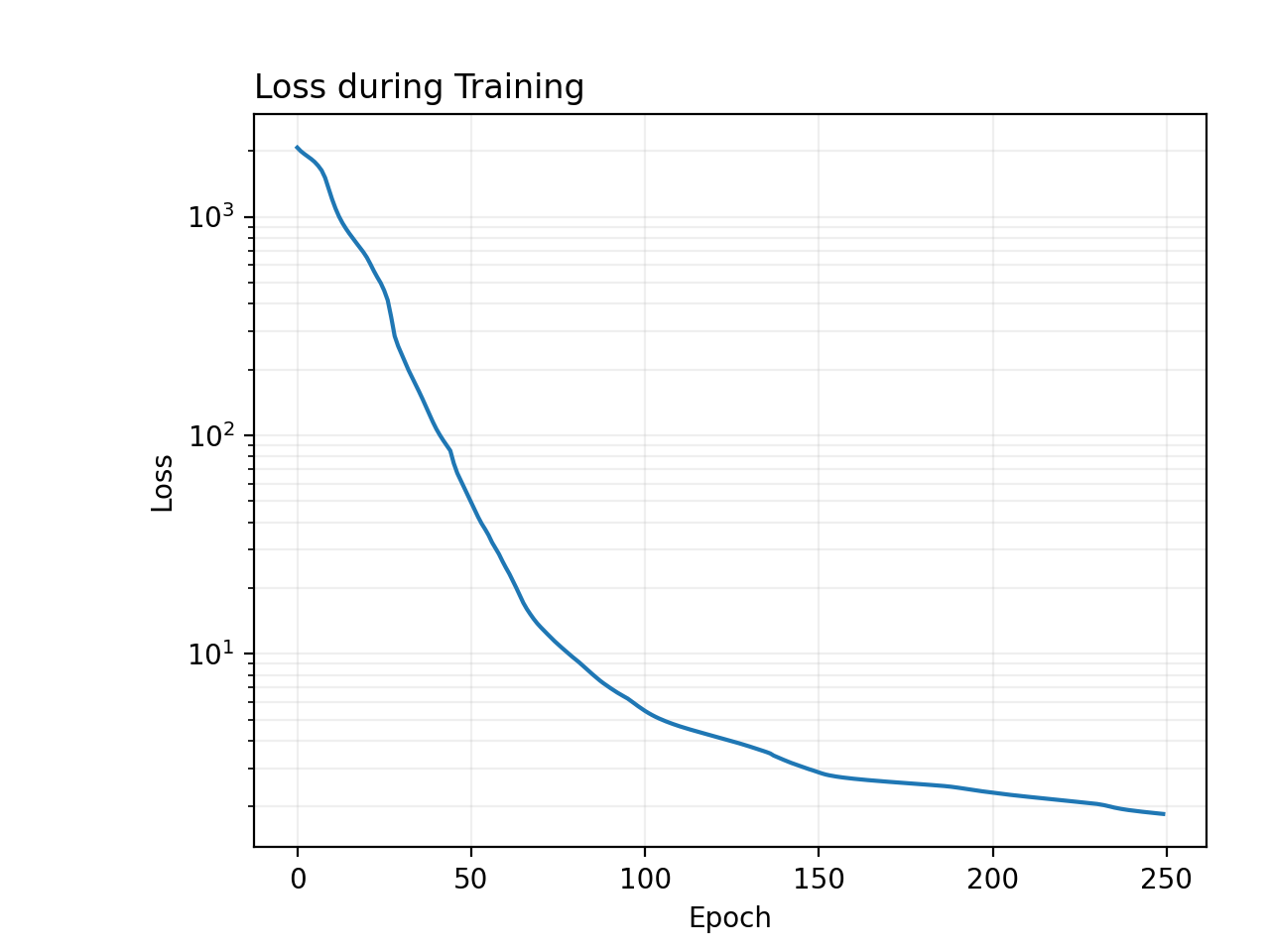
Resume training.
pinn.train(250)
# Visualize
pinn.plot_loss()
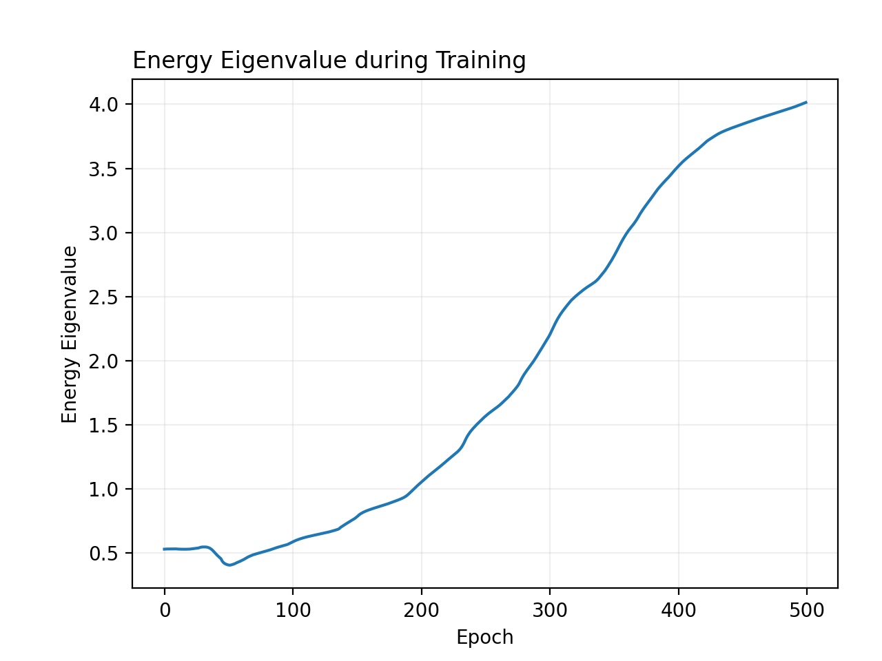
pinn.plot_energy()
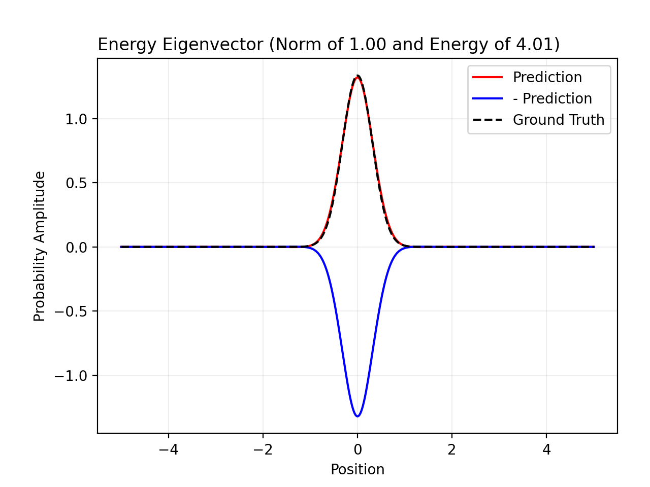
pinn.plot_wf(ref_wf=gnd_state)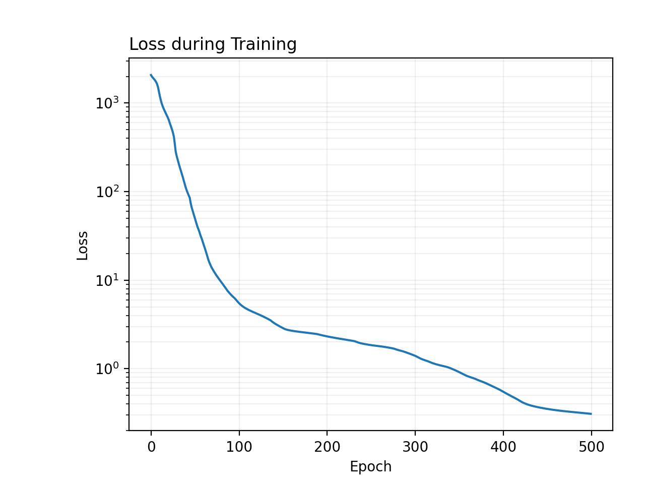
pinn.train(100)

# Visualize
pinn.animate(ref_energy=gnd_energy, ref_wf=gnd_state)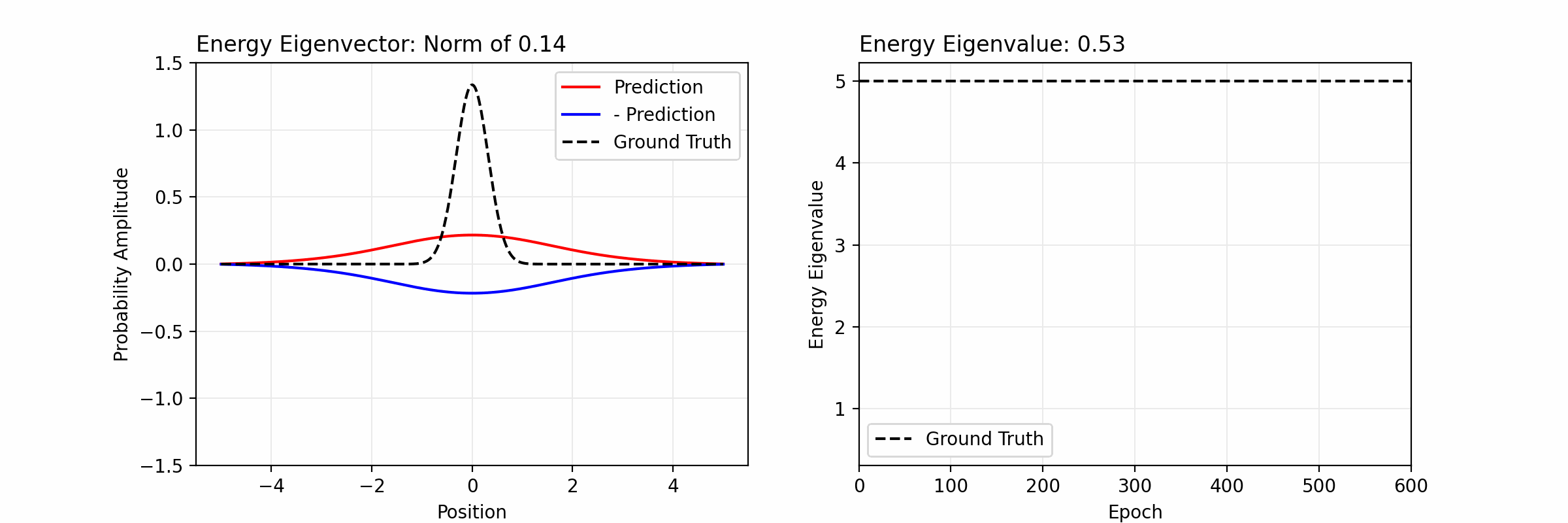
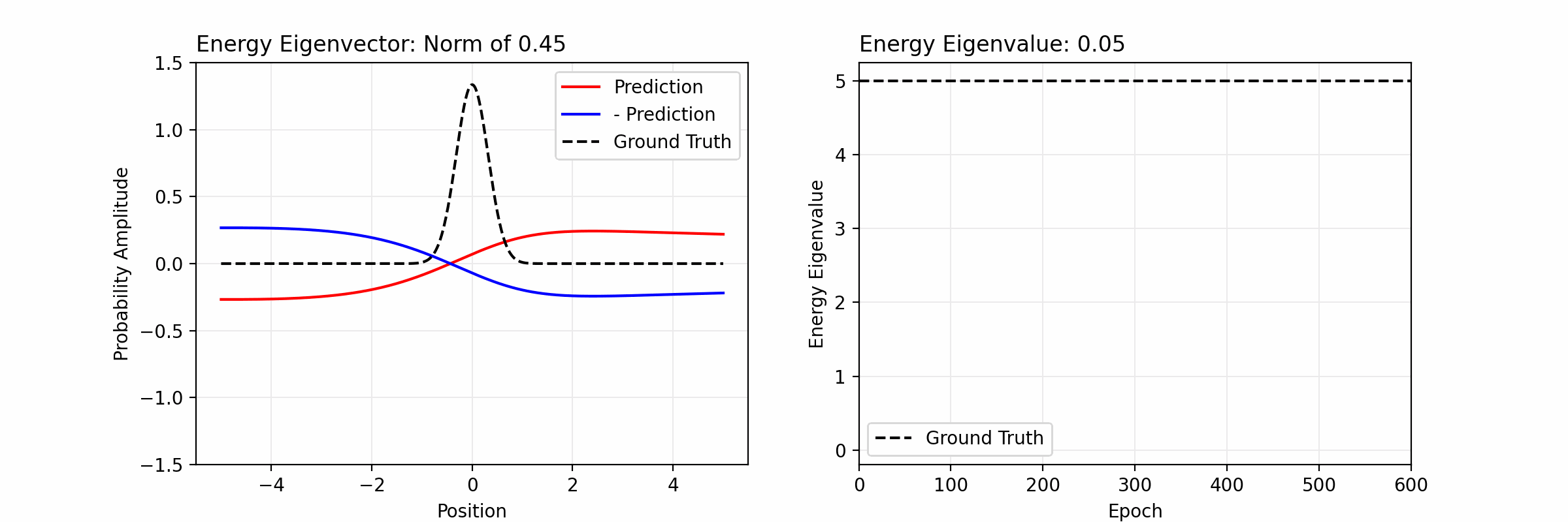
Compare with a PINN for which symmetry is not enforced.
params['sym'] = 0

pinn_without_sym = PINN(**params)
pinn_without_sym.init_optimizer('LBFGS', lr=1e-3)

pinn_without_sym.train(600)

pinn_without_sym.animate(ref_energy=gnd_energy, ref_wf=gnd_state)
Afterword
GitHub Repository
The repository for SE-PINN is hosted on GitHub at https://github.com/Tiger-Du/SE-PINN.
References
https://arxiv.org/abs/2203.00451
https://arxiv.org/abs/1904.08991